January 23, 2017 — 45 minutes read
math matrix
WARNING: Long article, big images, heavy GIFs.
A few weeks ago I was on an android-user-group channel,
when someone posted a question about Android’s
Matrix.postScale(sx, sy, px, py) method and how it works
because it was “hard to grasp”.
Coincidence: in the beginning of 2016, I finished a freelance project on an Android application where I had to implement an exciting feature:
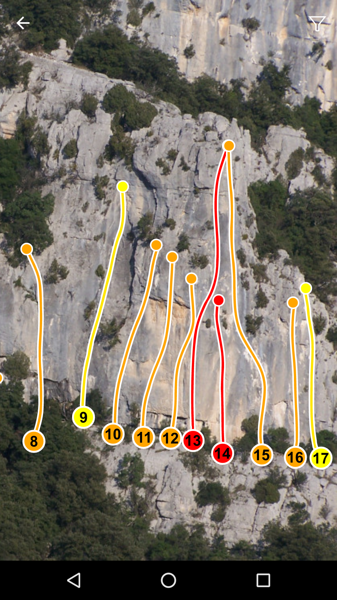
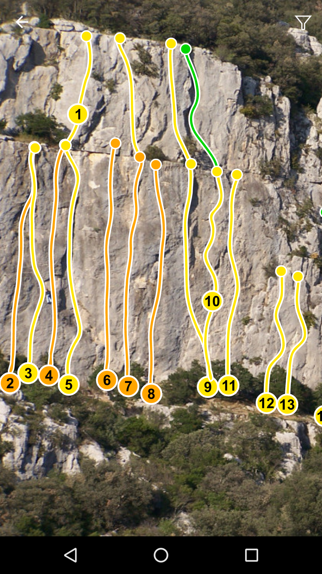
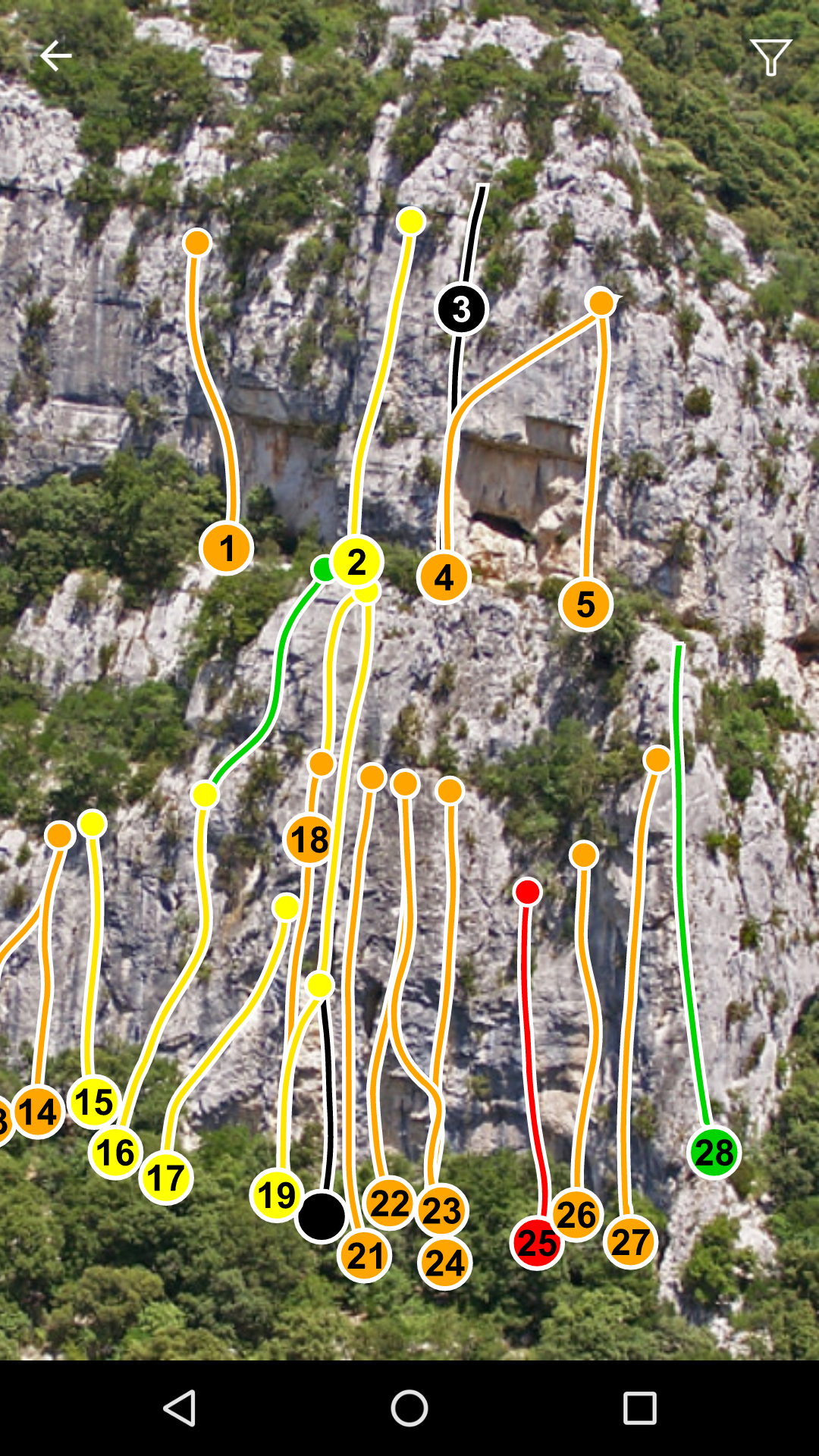
The user, after buying and downloading a digital topography of a crag, had to be able to view the crag which was composed of:
- a picture of the cliff,
- a SVG file containing an overlay of the climbing routes.
The user had to have the ability to pan and zoom at will and have the routes layer “follow” the picture.
Table Of Contents
Technical challenge
In order to have the overlay of routes follow the user’s actions, I found I
had to get my hands dirty by overloading an Android ImageView, draw onto the
Canvas and deal with finger gestures.
As a good engineer: I searched on Stack Overflow
:sweat_smile:
And I discovered I’d need the android.graphics.Matrix class for 2D
transformations.
The problem with this class, is that it might seem obvious what it does, but if you have no mathematical background, it’s quite mysterious.
boolean postScale (float sx, float sy, float px, float py)
Postconcats the matrix with the specified scale. M’ = S(sx, sy, px, py) * M
Yeah, cool, so it scales something with some parameters and it does it with some kind of multiplication. Nah, I don’t get it:
- What does it do exactly? Scales a matrix? What’s that supposed to mean, I want to scale the canvas…
- What should I use,
preScaleorpostScale? Do I try both while I get the input parameters from my gesture detection code and enter an infinite loop of trial and error guesstimates? (No. Fucking. Way.)
So at this very moment of the development process I realized I needed to re-learn basic math skills about matrices that I had forgotten many years ago, after finishing my first two years of uni :scream:
WWW to the rescue!
While searching around I’ve found a number of good resources and was able to learn some math again, and it felt great. It also helped me solve my 2D transformations problems by applying my understandings as code in Java and Android.
So, given the discussion I’ve had on the channel I’ve mentioned above, it seems I was not the only one struggling with matrices, trying to make sense of it and using these skills with Android’s Matrix class and methods, so I thought I’d write an article.
The first part, this one, is about matrices. The second part, “2D Transformations with Android and Java”, is about how to apply what you know about matrices in code, with Java and on Android.
What is a matrix?
The first resource you might encounter when trying to understand 2D transformations are articles about “Transformation matrix” and “Affine transformations” on Wikipedia:
- https://en.wikipedia.org/wiki/Transformation_matrix
- https://en.wikipedia.org/wiki/Transformation_matrix#Affine_transformations
- https://en.wikipedia.org/wiki/Affine_transformation
I don’t know you, but with this material, I almost got everything — wait…

NOPE! I didn’t get anything at all.
Luckily, on Khan Academy you will find a very well taught algebra course about matrices.
If you have this kind of problem, I encourage you to take the time needed to follow this course until you reach that “AHA” moment. It’s just a few hours of investment (it’s free) and you won’t regret it.
Why? Because matrices are good at representing data, and
operations on matrices can help you solve problems on this data. For instance,
remember having to solve systems of linear equations at school?
The most common ways (at least the two I‘ve studied) to solve a system
like that is with the elimination of variables method
or the row reduction method. But you can also use
matrices for that, which leads to interesting algorithms.
Matrices are used heavily in every branch of science, and they can also be
used for linear transformation to describe the position of points in space,
and this is the use case we will study in this article.
Anatomy
Simply put, a matrix is a 2D array. In fact, talking
about a $m \times n$ matrix relates to an array of length $m$ in which
each item is also an array but this time of length $n$. Usually, $m$
represents a rows’ number and $n$ a columns’ number. Each element in the
matrix is called an entry.
A matrix is represented by a bold capital letter,
and each entry is represented by the same letter, but in lowercase and suffixed
with its row number and column number, in this order. For example:
Now what can we do with it? We can define an algebra for instance: like addition, subtraction and multiplication operations, for fun and profit. :nerd:
Addition/Subtraction
Addition and subtraction of matrices is done by adding or subtracting the corresponding entries of the operand matrices:
Corollary to this definition we can deduce that in order to be defined, a matrix
addition or subtraction must be performed against two matrices of same
dimensions $m \times n$, otherwise the “corresponding entries” bit would
have no sense:
Grab a pen and paper and try to add a $3 \times 2$ matrix to a $2 \times 3$
matrix. What will you do with the last row of the first matrix? Same question
with the last column of the second matrix?
If you don’t know, then you’ve reached the same conclusion as the mathematicians
that defined matrices additions and subtractions, pretty much
:innocent:
Examples
Matrix multiplication
Throughout all my math schooling I’ve been said things like
"you can’t add apples to oranges, it makes no
sense”, in order to express the importance of units.
Well it turns out that multiplying apples and oranges is allowed.
And it can be applied to matrices: we can only add matrices to matrices, but
we can multiply matrices by numbers and by other matrices.
In the first case though, the number is not just a number (semantically). You don’t multiply a matrix by a number, you multiply a matrix by a scalar. In order to multiply a matrix by a scalar, we have to multiply each entry in the matrix by the scalar, which will give us another matrix as a result.
And a little example:
The second type of multiplication operation is the multiplication of matrices by matrices. This operation is a little bit more complicated than addition/subtraction because in order to multiply a matrix by a matrix we don’t simply multiply the corresponding entries. I’ll just quote wikipedia on that one:
:expressionless:if $\mathbf{A}$ is an $m \times n$ matrix and $\mathbf{B}$ is an $n \times p$ matrix, their matrix product $\mathbf{AB}$ is an $m \times p$ matrix, in which the $n$ entries across a row of $\mathbf{A}$ are multiplied with the $n$ entries down a columns of $\mathbf{B}$ and summed to produce an entry of $\mathbf{AB}$
This hurts my brain, let’s break it down:
if $\mathbf{A}$ is an $m \times n$ matrix and $\mathbf{B}$ is an $n \times p$ matrix, their matrix product $\mathbf{AB}$ is an $m \times p$ matrix
We can write this in a more graphical way: $ {\tiny\begin{matrix}^{\scriptsize }\\ \normalsize \mathbf{A} \\ ^{\scriptsize m \times n}\end{matrix} } \times {\tiny\begin{matrix}^{\scriptsize }\\ \normalsize \mathbf{B} \\ ^{\scriptsize n \times p}\end{matrix} } = {\tiny\begin{matrix}^{\scriptsize }\\ \normalsize \mathbf{AB} \\ ^{\scriptsize m \times p}\end{matrix} } $.
See this simple matrix
$
{\tiny\begin{matrix}^{\scriptsize }\\ \normalsize \mathbf{A} \\ ^{\scriptsize 2 \times 3}\end{matrix} } =
\begin{pmatrix}a_{11} & a_{12} & a_{13}\\a_{21} & a_{22} & a_{23}\end{pmatrix}
$
and this other matrix
$
{\tiny\begin{matrix}^{\scriptsize }\\ \normalsize \mathbf{B} \\ ^{\scriptsize 3 \times 1}\end{matrix} } =
\begin{pmatrix}b_{11}\\b_{21}\\b_{31}\end{pmatrix}
$.
We have $m=2$, $n=3$ and $p=1$ so the multiplication will give
$
{\tiny\begin{matrix}^{\scriptsize }\\ \normalsize \mathbf{AB} \\ ^{\scriptsize 2 \times 1}\end{matrix} } =
\begin{pmatrix}ab_{11}\\ab_{21}\end{pmatrix}
$.
Let’s decompose the second part now:
- “the $n$ entries across a row of $\mathbf{A}$” means that each row in $\mathbf{A}$ is an array of $n=3$ entries: if we take the first row we get $a_{11}$, $a_{12}$ and $a_{13}$.
- “the $n$ entries down a columns of $\mathbf{B}$” means that each column of $\mathbf{B}$ is also an array of $n=3$ entries: in the first column we get $b_{11}$, $b_{21}$ and $b_{31}$.
- “are multiplied with” means that each entry in $\mathbf{A}$'s row must be multiplied with its corresponding (first with first, second with second, etc.) entry in $\mathbf{B}$'s column: $a_{11} \times b_{11}$, $a_{12} \times b_{21}$ and $a_{13} \times b_{31}$
- “And summed to produce an entry of $\mathbf{AB}$” means that we must add the products of these corresponding rows and columns entries in order to get the entry of the new matrix at this row number and column number: in our case we took the products of the entries in the first row in the first matrix with the entries in the first column in the second matrix, so this will give us the entry in the first row and first column of the new matrix: $a_{11} \times b_{11} + a_{12} \times b_{21} + a_{13} \times b_{31}$
To plagiate wikipedia, here is the formula:
Ok I realize I don’t have any better way to explain this so here is a visual representation of the matrix multiplication process and an example:

Remember:
In order for matrix multiplication to be defined, the number of columns in the first matrix must be equal to the number of rows in the second matrix.
Otherwise you can’t multiply, period.
More details here and here if you are interested.
Transformation matrices
Now that we know what is a matrix and how we can multiply matrices, we can see why it is interesting for 2D transformations.
Transforming points
As I’ve said previously, matrices can be used to represent systems of linear equations. Suppose I give you this system:
Now that you are familiar with matrix multiplications, maybe you can see this coming, but we can definitely express this system of equations as the following matrix multiplication:
If we go a little further, we can see something else based on the matrices
$\begin{pmatrix}x\\y\end{pmatrix}$ and
$\begin{pmatrix}5\\0\end{pmatrix}$.
We can see that they can be used to reprensent points in the Cartesian
plane, right? A point can be represented by a vector originating from origin,
and a vector is just a $2 \times 1$ matrix.
What we have here, is a matrix multiplication that represents the transformation of a point into another point. We don’t know what the first point’s coordinates are yet, and it doesn’t matter. What I wanted to show is that, given a position vector, we are able to transform it into another via a matrix multiplication operation.
Given a point $P$, whose coordinates are represented by the position vector, $\begin{pmatrix}x\\y\end{pmatrix}$, we can obtain a new point $P^{\prime}$ whose coordinates are represented by the position vector $\begin{pmatrix}x^{\prime}\\y^{\prime}\end{pmatrix}$ by multiplying it by a matrix.
One important thing is that this transformation matrix has to have specific dimensions, in order to fulfill the rule of matrix multiplication: because $\begin{pmatrix}x\\y\end{pmatrix}$ is a $2 \times 1$ matrix, and $\begin{pmatrix}x^{\prime}\\y^{\prime}\end{pmatrix}$ is also a $2 \times 1$ matrix, then the transformation matrix has to be a $2 \times 2$ matrix in order to have:
Note: The order here is important as we will see later, but you can already see that switching $\mathbf{A}$ and $\begin{pmatrix}x\\y\end{pmatrix}$ would lead to an $undefined$ result (if you don’t get it, re-read the part on matrix multiplication and their dimensions).
Notice that the nature of the transformation represented by our matrix above and in the link is not clear, and I didn’t say what kind of transformation it is, on purpose. The transformation matrix was picked at random, and yet we see how interesting and useful it is for 2D manipulation of graphics.
Another great thing about transformation matrices, is that they can be used to transform a whole bunch of points at the same time.
For now, I suppose all you know is the type of transformations you want to
apply: rotation, scale or translation and some parameters.
So how do you go from scale by a factor of 2 and rotate 90 degrees clockwise
to a transformation matrix?
Well the answer is:

More math stuff
More specifically I encourage you to read this course on Matrices as transformations (which is full of fancy plots and animations) and particularly its last part: Representing two dimensional linear transforms with matrices.
Come back here once you’ve read it, or it’s goind to hurt :sweat_smile:
Ok I suppose you’ve read the course above, but just in case, here is a reminder
- a position vector $\begin{pmatrix}x\\y\end{pmatrix}$ can be broken down as $\begin{pmatrix}x\\y\end{pmatrix} = x.\begin{pmatrix}\color{Green} 1\\ \color{Green} 0\end{pmatrix} + y.\begin{pmatrix}\color{Red} 0\\ \color{Red} 1\end{pmatrix}$.
- $\begin{pmatrix}\color{Green} a\\ \color{Green} c\end{pmatrix}$ and $\begin{pmatrix}\color{Red} b\\ \color{Red} d\end{pmatrix}$ are the position vectors where $\begin{pmatrix} \color{Green} 0\\ \color{Green} 1\end{pmatrix}$ and $\begin{pmatrix} \color{Red} 1\\ \color{Red} 0\end{pmatrix}$ will land respectively after the transformation matrix $\mathbf{A} = \begin{pmatrix} \color{Green} a & \color{Red} b\\ \color{Green} c & \color{Red} d \end{pmatrix}$ has been applied.
- given the previous transformation, $\begin{pmatrix} x\\ y \end{pmatrix}$ will land on $\begin{pmatrix} \color{Green} a.x + \color{Red} b.y\\ \color{Green} c.x + \color{Red} d.y \end{pmatrix}$.
If you don’t understand this conclusion, read again, read the course, take your time.
Now remember, our goal is to determine what $ \mathbf{A} $ is, because we know the transformation we want to apply but we’re searching for the matrix we should apply to our position vector(s) in order to transform our graphics.
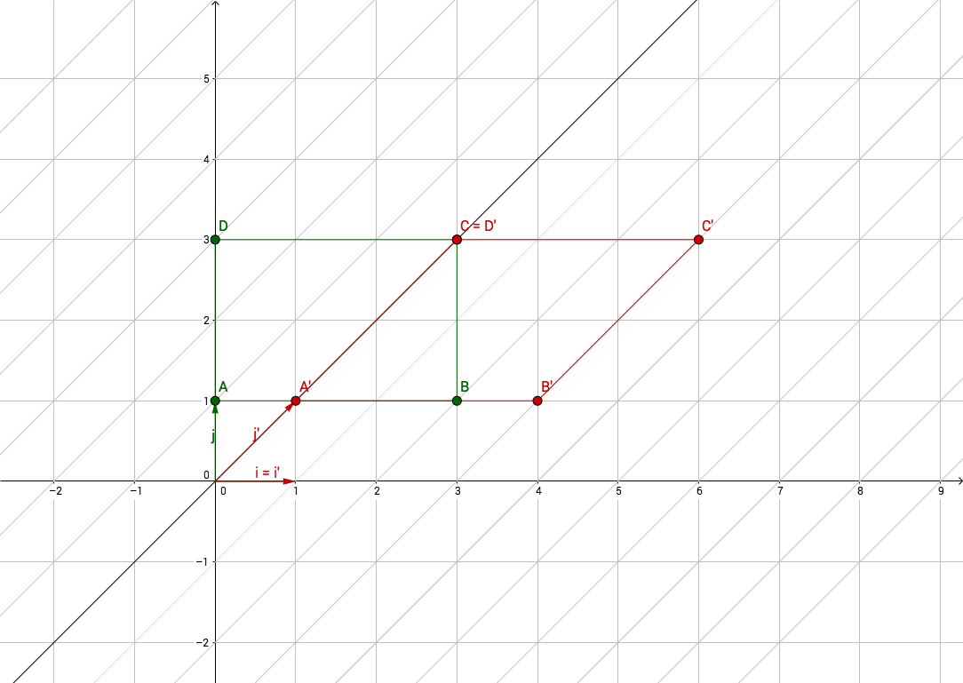
Let’s take the example of the transformation of a series of points: we know
where the position vectors will land, but we’re looking for $ \mathbf{A} $.
We have our cartesian plane with a triangle formed by the three points
$P_{(2,1)}$, $Q_{(-2,0)}$, $R_{(0,2)}$, and another triangle which
represents a transformed version of the first one: $P^{\prime}_{(5, 0)}$
and $Q^{\prime}_{(-4, 2)}$ and $R^{\prime}_{(2,4)}$.
We just need two points for this example, let’s take $P$ and $Q$. We know that:
Which means:
From which we can deduce:
The right side gives us $ a=2 $ and $ c = -1 $, with which we can deduce $ b=1 $ and $ d=2 $ from the left side.
And this, is our transformation matrix:
Try that same exercise with $P$ and $R$, or with $Q$ and $R$ and you should end up to the same result.
The identity matrix
We don’t know how to define a transformation matrix yet, but we know its form.
So what do we do next? Remember the last section where we’ve seen that
a position vector $\begin{pmatrix} x\\ y \end{pmatrix}$ can be
broken down as $\begin{pmatrix} x\\y \end{pmatrix} =
x.\begin{pmatrix} \color{Green} 1\\ \color{Green} 0 \end{pmatrix} +
y.\begin{pmatrix} \color{Red} 0\\ \color{Red} 1 \end{pmatrix} $
?
That’s a pretty good starting point, we just laid out our “base” matrix:
This matrix represents the base state of your plane, the matrix applied
to your plane when you have just loaded your image for example (granted
your image is the same size as its receiving container view).
In other words, this is the matrix that, applied to any position vector will
return that same position vector.
This matrix is called the identity matrix.
Combining transformations
One more thing before we get concrete: We want our user to be able to combine/chain transformations (like zooming and panning at the same time for instance).
In order to chain multiple transformations we need to understand the
properties of matrix multiplication, and more
specifically the non-commutative and associative properties of matrix
multiplication:
- Matrix multiplication is associative $\left(\mathbf{A}.\mathbf{B}\right).\mathbf{C} = \mathbf{A}.\left(\mathbf{B}.\mathbf{C}\right)$
- Matrix multiplication is non-commutative $\mathbf{A}.\mathbf{B} \neq \mathbf{B}.\mathbf{A}$
Back to our transformations.
Imagine we want to apply transformation $ \mathbf{B} $, then transformation
$ \mathbf{A} $ to our position vector $ \vec{v} $.
We have $ \vec{v^{\prime}} = \mathbf{B} . \vec{v} $ and $ \vec{v^{\prime\prime}} = \mathbf{A} . \vec{v^{\prime}} $, which leads us to:
We know that matrix multiplication is associative, which gives us:
In conclusion, in order to apply multiple transformations at once, we can multiply all our transformation matrices and apply the resulting transformation matrix to our vector(s).
We also know that matrix multiplication is not commutative, so the order
in which we multiply our transformation matrices
($ \mathbf{A} . \mathbf{B} $ or $ \mathbf{B} . \mathbf{A} $) will have
an impact on our final matrix and will lead to different results, different
transformations.
Types of transformations
There are several types of 2D transformations we are able to define using
$2 \times 2$ dimensions matrices, and you’ve had a preview of most of them
in this course on matrices as transformations.
Namely:
- Scaling
- Reflexion
- Shearing
- Rotation
For the rest of this section imagine we have the point $ P_{\left(x, y\right)} $, which represents any point of an object on the plane, and we want to find the matrix to transform it into $ P^{\prime}_{\left(x^{\prime}, y^{\prime}\right)}$ such that
Scaling
Scaling (like zooming in by a factor of 2 for instance) might seem
straightforward to represent, right?
“Simply multiply the coordinates by the scaling factor and you’re done."
But the pitfall here is that you might want to have different horizontal and
vertical scaling factors for your transformation, I mean it’s possible!
So we must differentiate between $ s_{x} $ and $ s_{y} $ which represent the horizontal and vertical scaling factors, respectively.
The two equations this gives us are:
Knowing that:
We can find $a$, $b$, $c$ and $d$:
In conclusion, the $2 \times 2$ scaling matrix for the factors $\left(s_{x}, s_{y}\right)$ is:
Which makes sense, right? I mean, scaling by a factor of $1$ both on the $x$ and $y$ axises will give:
Which is… the identity matrix! So nothing moves, basically.
Reflexion
There are 2 types of reflexions we can think about right ahead: reflexion around
an axis, or around a point.
To keep things simple we’ll focus on reflexions around the $x$ and $y$
axises (reflexion around the origin is the equivalent of applying a reflexion on
the $x$ and $y$ axises successively).
Reflexion around the $x$ axis gives us:
Funny, reflecting around the $x$ axis is the same transformation as scaling $x$ by a factor of $-1$ and $y$ by a factor of $1$:
And reflexion around the $y$ axis gives us:
The transformation matrix to reflect around the $y$ axis is:
Shearing
Now it gets a little bit trickier.
In most examples I’ve found, shearing is explained by saying the coordinates
are changed by adding a constant that measures the degree of shearing.
For instance, a shear along the $x$ axis is often represented showing a
rectangle with a vertex at $\left(0, 1\right)$ is transformed into a
parallelogram with a vertex at $\left(1, 1\right)$.
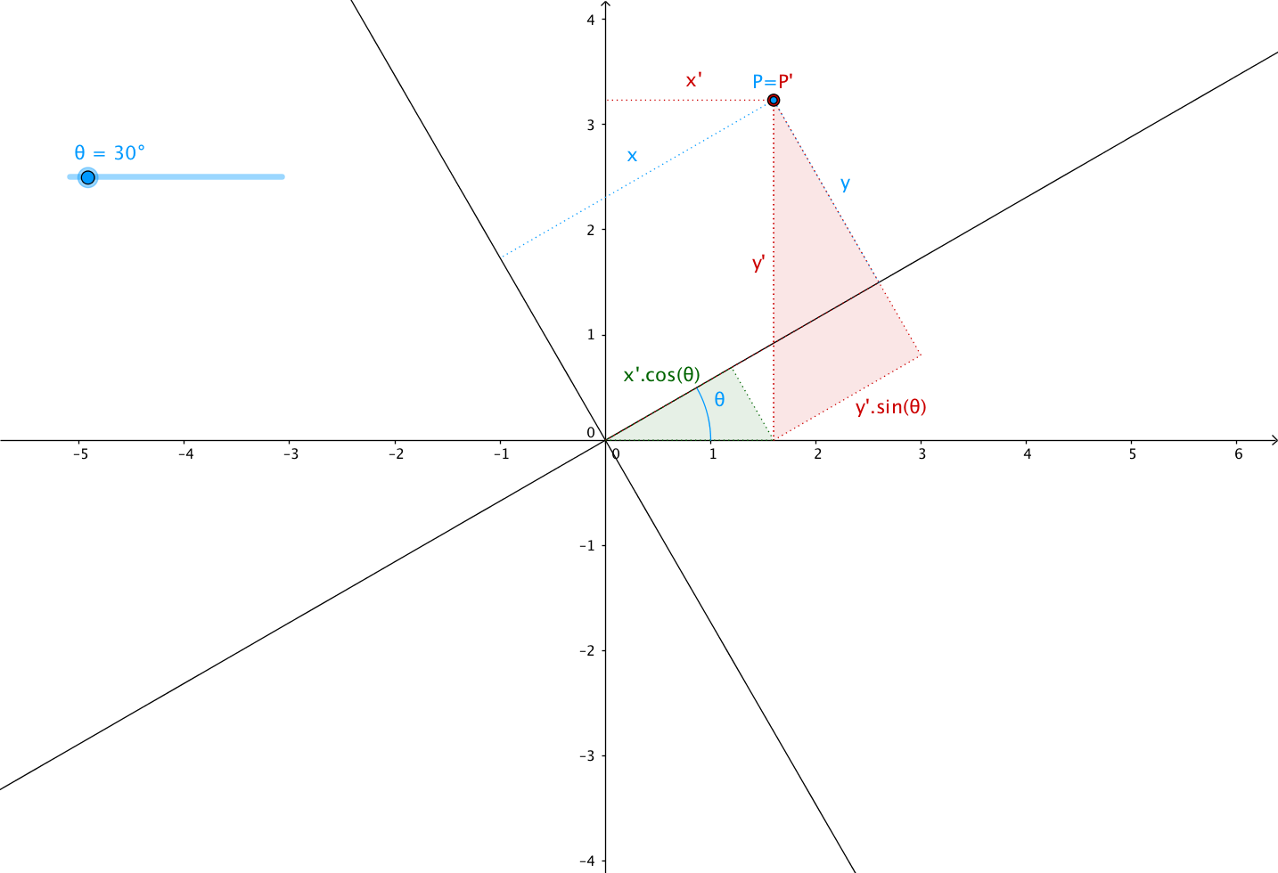
In this article, I want to explain it using the shearing angle, the angle through which the axis is sheared. Let’s call it $\alpha$ (alpha).
If we look at the plane above, we can see that the new abscissa $x^{\prime}$ is equal to $x$ plus/minus the opposite side of the triangle formed by the $y$ axis, the sheared version of the $y$ axis and the segment between the top left vertex of the rectangle and the top left vertex of the parallelogram. In other words, $x^{\prime}$ is equal to $x$ plus/minus the opposite side of the green triangle, see:
>0")
>0")
<0")
<0")
Remember your trigonometry class?
In a right-angled triangle:
- the hypotenuse is the longest side
- the opposite side is the one at the opposite of a given angle
- the adjacent side is the next to a given angle
- $PP^{\prime}$ is the opposite side, we need to find its length ($k$), in order to calculate $x^{\prime}$ from $x$
- the adjacent side is $P$'s ordinate: $y$
- we don’t know the hypotenuse’s length
From our trigonometry class, we know that:
We know $\alpha$, but we don’t know the length of the hypotenuse, so we
can’t use the cosine function.
On the other hand, we know the adjacent side’s length: it’s $y$, so we can use
the tangent function to find the opposite side’s length:
We can start solving our system of equations in order to find our matrix with the following:
However, we can see that when $\alpha > 0$, $\tan \left( \alpha \right) < 0$ and
when $\alpha < 0$, $\tan \left( \alpha \right) > 0$. This multiplied by $y$
which can itself be positive or negative will give very different results
for $x^{\prime} = x + k = x + y . \tan \left( \alpha \right)$.
So don’t forget that $\alpha > 0$ is counterclockwise rotation/shearing angle,
while $\alpha < 0$ is clockwise rotation/shearing angle.
The transformation matrix to shear along the $x$ direction is:
Similarly, the transformation matrix to shear along the $y$ direction is:
Rotation
Rotations are yet a little bit more complex.
Let’s take a closer look at it with an example of rotating (around the origin) from a angle $ \theta $ (theta).

Notice how the coordinates of $P$ and $P^{\prime}$ are the same in their
respective planes:
$P$ and $P^{\prime}$ have the same set of coordinates $ \left( x, y\right) $
in each planes.
But $P^{\prime}$ has new coordinates
$ \left( x^{\prime}, y^{\prime}\right) $ in the first plane, the one that
has not been rotated.
We can now define the relationship between the coordinates $ \left(x, y\right) $ and the new coordinates $ \left(x^{\prime}, y^{\prime}\right) $, right?
This is where trigonometry helps again.
While searching for the demonstration of this, I stumbled upon this geometry based explanation by Nick Berry and this video.
To be honest, I’m not 100% comfortable with this solution, which means I didn’t
fully understand it. And also after re-reading what I’ve written, Hadrien
(one of the reviewers) and I have found my explanation to be a bit
awkward.
So I’m leaving it here in case you’re interested, but I suggest you
don’t bother unless you’re very curious and don’t mind a little confusion.
Now for the simple demonstration I’m going to go with the “This position vector lands on this position vector” route.
Suppose you are zooming on the unit vectors like so:
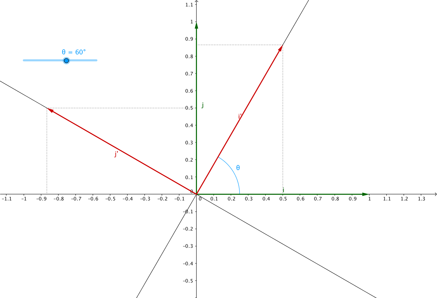
Based on the rules of trigonometry we’ve already seen, we have:
Which means:
From which we can deduce:
Easy to deduce $ a = \cos \left( \theta \right) $, $ b = - \sin \left( \theta \right) $, $ c = \sin \left( \theta \right) $ and $ d = \cos \left( \theta \right) $.
Which gives us our desired rotation matrix:
Congratulations! You know of to define scaling, reflexion, shearing and rotation transformation matrices. So what is missing?
3x3 transformation matrices
If you’re still with me at this point, maybe you’re wondering why any of this is useful. If it’s the case, you missed the point of this article, which is to understand affine transformations in order to apply them in code :mortar_board: .
This is useful because at this point you know what a transformation matrix looks like, and you know how to compute one given a few position vectors, and it is also a great accomplishment by itself.
But here’s the thing: $2 \times 2$ matrices are limited in the number of operations we can perform. With a $2 \times 2$ matrix, the only transformations we can do are the ones we’ve seen in the previous section:
- Scaling
- Reflexion
- Shearing
- Rotation
So what are we missing? Answer: translations!
And this is unfortunate, as translations are really useful, like when the user
pans and the image has to behave accordingly (aka. follow the finger).
Translations are defined by the addition of two matrices :
But we want our user to be able to combine/chain transformations (like zooming on a specific point which is not the origin), so we need to find a way to express translations as matrices multiplications too.
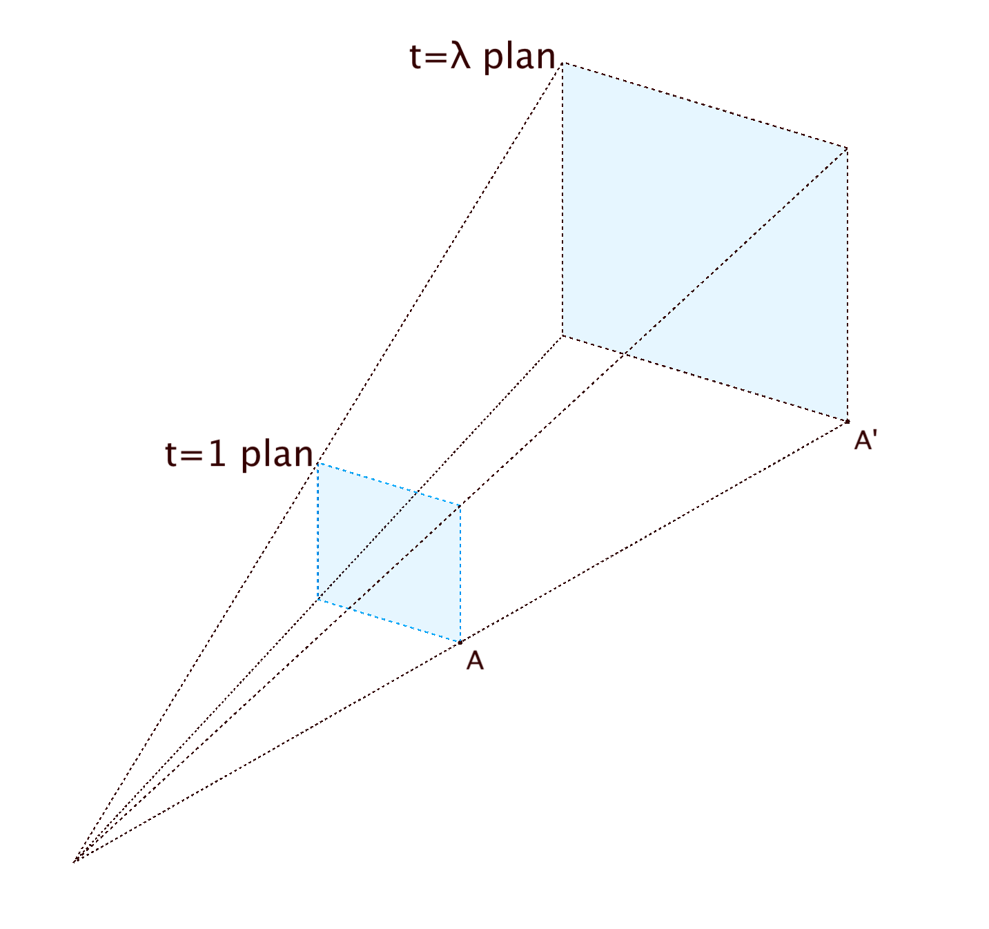
Here comes the world of Homogeneous coordinates…
No, you don’t have to read it, and no I don’t totally get it either…
The gist of it is:
- the Cartesian plane you’re used to, is really just one of many planes that exist in the 3D space, and is at $ z = 1 $
- for any point $ \left(x, y, z\right)$ in the 3D space, the line in the projecting space that is going through this point and the origin is also passing through any point that is obtained by scaling $x$, $y$ and $z$ by the same factor
- the coordinates of any of these points on the line is $ \left(\frac{x}{z}, \frac{y}{z}, z\right)$.
I’ve collected a list of blog posts, articles and videos links at the end of this post if you’re interested.
Without further dig in, this is helping, because it says that we can now represent any point in our Cartesian plane ($ z = 1 $) not only as a $2 \times 1$ matrix, but also as a $3 \times 1$ matrix:
Which means we have to redefine all our previous transformation matrices,
because the product of a $3 \times 1$ matrix (position vector) by a
$2 \times 2$ matrix (transformation) is undefined.
Don’t rage quit! It’s straightforward: $\mathbf{z^{\prime}=z}$!
We have to find the transformation matrix $ \mathbf{A} = \begin{pmatrix} a & b & c\\ d & e & f\\ g & h & i \end{pmatrix} $
If, like in the previous section, we imagine that we have the point $ P_{\left(x, y, z\right)} $, which represents any point of an object on the cartesian plane, then we want to find the matrix to transform it into $ P^{\prime}_{\left(x^{\prime}, y^{\prime}, z^{\prime}\right)}$ such that
Scaling
We are looking for $\mathbf{A}$ such that:
We can solve the following system of equation in order to find $\mathbf{A}$:
The 3x3 scaling matrix for the factors $ \left(s_{x}, s_{y}\right) $ is:
Reflexion
For a reflexion around the $x$ axis we are looking for $\mathbf{A}$ such that:
We can solve the following system of equation in order to find $\mathbf{A}$:
The transformation matrix to reflect around the $x$ axis is:
For the reflexion around the $y$ axis we are looking for $\mathbf{A}$ such that:
We can solve the following system of equation in order to find $\mathbf{A}$:
The transformation matrix to reflect around the $y$ axis is:
Shearing
Well, I’m a bit lazy here :hugging:
You see the pattern, right? Third line always the same, third column always the same.
The transformation matrix to shear along the $x$ direction is:
Similarly, the transformation matrix to shear along the $y$ direction is:
Rotating
Same pattern, basically we just take the $2 \times 2$ rotation matrix and add one row and one column whose entries are $0$, $0$ and $1$.
But you can do the math, if you want :stuck_out_tongue_winking_eye:
Translation
And now it gets interesting, because we can define translations as $3 \times 3$ matrices multiplication!
We are looking for $\mathbf{A}$ such that:
We can solve the following system of equation in order to find $\mathbf{A}$:
The $3 \times 3$ translation matrix for the translation $ \left(t_{x}, t_{y}\right) $ is:
Matrices wrap-up
Obviously, you won’t have to go into all of these algebra stuff each time you want to know what is the matrix you need to apply in order to do your transformations.
You can just use the following:
Reminder
Translation matrix: $\begin{pmatrix}1 & 0 & t_{x}\\0 & 1 & t_{y}\\0 & 0 & 1\end{pmatrix}$
Scaling matrix: $\begin{pmatrix}s_{x} & 0 & 0\\0 & s_{y} & 0\\0 & 0 & 1\end{pmatrix}$
Shear matrix: $\begin{pmatrix}1 & \tan \alpha & 0\\\tan \beta & 1 & 0\\0 & 0 & 1\end{pmatrix} = \begin{pmatrix}1 & k_{x} & 0\\k_{y} & 1 & 0\\0 & 0 & 1\end{pmatrix}$
Rotation matrix: $\begin{pmatrix}\cos \theta & -\sin \theta & 0\\\sin \theta & \cos \theta & 0\\0 & 0 & 1\end{pmatrix}$
That’s neat! Now you can define your matrices easily, plus you know how it works.
One last thing: all the transformations we’ve seen are centered around the
origin.
How do we apply what we know in order to, for instance, zoom on a
specific point which is not the origin, or rotate an object in place,
around its center?
The answer is composition: We must compose our transformations by using several other transformations.
Combination use-case: pinch-zoom
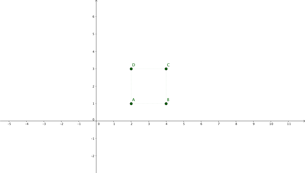
Imagine you have a shape, like a square for instance, and you want to zoom in at the center of the square, to mimic a pinch-zoom behaviour :mag:
This transformation is composed of the following sequence:
- move anchor point to origin: $ \left( -t_{x}, -t_{y} \right) $
- scale by $ \left( s_{x}, s_{y} \right) $
- move back anchor point: $ \left( t_{x}, t_{y} \right) $
Where $t$ is the anchor point of our scaling transformation (the center of the square).
Our transformations are defined by the first translation matrix $ \mathbf{C} $, the scaling matrix $ \mathbf{B} $, and the last translation matrix $ \mathbf{A} $.
Because matrix multiplication is non-commutative, the order matters, so we will
apply them in reverse order (hence the reverse naming order).
The composition of these transformations gives us the following product:
Suppose we have the following points representing a square: $\begin{pmatrix}x_{1} & x_{2} & x_{3} & x_{4}\\y_{1} & y_{2} & y_{3} & y_{4}\\1 & 1 & 1 & 1\end{pmatrix} = \begin{pmatrix}2 & 4 & 4 & 2\\1 & 1 & 3 & 3\\1 & 1 & 1 & 1\end{pmatrix}$

And we want to apply a 2x zoom focusing on its center.
The new coordinates will be:
Combination use-case: rotate image
Now imagine you have an image in a view, the origin is not a the center of the view, it is probably at the top-left corner (implementations may vary), but you want to rotate the image at the center of the view :upside_down:
This transformation is composed of the following sequence:
- move anchor point to origin: $ \left( -t_{x}, -t_{y} \right) $
- rotate by $ \theta $
- move back anchor point: $ \left( t_{x}, t_{y} \right) $
Where $t$ is the anchor point of our rotation transformation.
Our transformations are defined by the first translation matrix $ \mathbf{C} $, the rotation matrix $ \mathbf{B} $, and the last translation matrix $ \mathbf{A} $.
The composition of these transformations gives us the following product:
Suppose we have the following points representing a square: $\begin{pmatrix}x_{1} & x_{2} & x_{3} & x_{4}\\y_{1} & y_{2} & y_{3} & y_{4}\\1 & 1 & 1 & 1\end{pmatrix} = \begin{pmatrix}2 & 4 & 4 & 2\\1 & 1 & 3 & 3\\1 & 1 & 1 & 1\end{pmatrix}$
And we want to apply a rotation of $ \theta = 90^{\circ} $ focusing on its center.
The new coordinates will be:
Acknowledgements
I want to address my warmest thank you to the following people, who helped me during the review process of this article, by providing helpful feedbacks and advices:
- Igor Laborie (@ilaborie)
- Hadrien Toma (@HadrienToma)
Resources
Links
- Khan Academy algebra course on matrices
- A course on “Affine Transformation” at The University of Texas at Austin
- A course on “Composing Transformations” at The Ohio State University
- A blogpost on “Rotating images” by Nick Berry
- A Youtube video course on “The Rotation Matrix” by Michael J. Ruiz
- Wikipedia on Homogeneous coordinates
- A blogpost on “Explaining Homogeneous Coordinates & Projective Geometry” by Tom Dalling
- A blogpost on “Homogeneous Coordinates” by Song Ho Ahn
- A Youtube video course on “2D transformations and homogeneous coordinates” by Tarun Gehlot
This blog uses Hypothesis for public and private (group) comments.
You can annotate or highlight words or paragraphs directly by selecting the text!
If you want to leave a general comment or read what others have to say, please use the collapsible panel on the right of this page.